Error function
In-game article clicks load inline without leaving the challenge.
In mathematics, the error function (also called the Gauss error function), often denoted by e r f {\displaystyle \mathbf {erf} }, is the function erf ( z ) = 2 π ∫ 0 z e − t 2 d t . {\displaystyle \operatorname {erf} (z)={\frac {2}{\sqrt {\pi }}}\int _{0}^{z}e^{-t^{2}}\,dt.}
The integral here is a complex contour integral which is path-independent because exp ( − t 2 ) {\displaystyle \exp(-t^{2})} is holomorphic on the whole complex plane C {\displaystyle \mathbb {C} }. In many applications, the function argument is a real number, in which case the function value is also real.
In some older texts, the error function is defined without the factor of 2 / π {\displaystyle 2/{\sqrt {\pi }}}. This nonelementary integral is a sigmoid function that occurs often in probability, statistics, and partial differential equations.
In statistics, for non-negative real values of X {\displaystyle X}, the error function has the following interpretation: for a real random variable Y {\displaystyle Y} that is normally distributed with mean 0 and standard deviation 1 / 2 {\displaystyle 1/{\sqrt {2}}}, erf ( x ) {\displaystyle \operatorname {erf} (x)} is the probability that Y {\displaystyle Y} falls in the range [ − x , x ] {\displaystyle [-x,x]}.
Two closely related functions are the complementary error function
erfc ( z ) = 1 − erf ( z ) {\displaystyle \operatorname {erfc} (z)=1-\operatorname {erf} (z)}
and the imaginary error function
erfi ( z ) = − i erf ( i z ) , {\displaystyle \operatorname {erfi} (z)=-i\operatorname {erf} (iz),}
where i {\displaystyle i} is the imaginary unit.
Name
The name "error function" and its abbreviation erf {\displaystyle \operatorname {erf} } were proposed by J. W. L. Glaisher in 1871 on account of its connection with "the theory of probability, and notably the theory of errors". The complementary error function was also discussed by Glaisher in a separate publication in the same year. For the "law of facility" of errors whose density is given by
f ( x ) = ( c π ) 1 / 2 e − c x 2 {\displaystyle f(x)=\left({\frac {c}{\pi }}\right)^{1/2}e^{-cx^{2}}}
(the normal distribution), Glaisher calculates the probability of an error lying between p {\displaystyle p} and q {\displaystyle q} as
( c π ) 1 2 ∫ p q e − c x 2 d x = 1 2 ( erf ( q c ) − erf ( p c ) ) . {\displaystyle \left({\frac {c}{\pi }}\right)^{\frac {1}{2}}\int _{p}^{q}e^{-cx^{2}}\,dx={\frac {1}{2}}{\big (}\operatorname {erf} (q{\sqrt {c}})-\operatorname {erf} (p{\sqrt {c}}){\big )}.}
Applications
When the results of a series of measurements are described by a normal distribution with standard deviation σ {\displaystyle \sigma } and expected value zero, then
erf ( a σ 2 ) {\displaystyle \operatorname {erf} {\bigg (}{\frac {a}{\sigma {\sqrt {2}}}}{\bigg )}}
is the probability that the error of a single measurement lies between − a {\displaystyle -a} and a {\displaystyle a}. This is useful, for example, in determining the bit error rate of a digital communication system.
The error and complementary error functions occur, for example, in solutions of the heat equation when boundary conditions are given by the Heaviside step function.
The error function and its approximations can be used to estimate results that hold with high probability or with low probability. Given a normally distributed random variable X {\displaystyle X} with mean μ {\displaystyle \mu } and standard deviation σ {\displaystyle \sigma } and a constant L > μ {\displaystyle L>\mu }, it can be shown (via integration by substitution) that
Pr [ X ≤ L ] = 1 2 + 1 2 erf ( L − μ 2 σ ) ≈ A exp ( − B ( L − μ σ ) 2 ) {\displaystyle \Pr[X\leq L]={\frac {1}{2}}+{\frac {1}{2}}\operatorname {erf} \left({\frac {L-\mu }{{\sqrt {2}}\sigma }}\right)\approx A\exp \left(\!-B\,\left({\frac {L-\mu }{\sigma }}\right)^{2}\right)}
where A {\displaystyle A} and B {\displaystyle B} are certain numeric constants. If L {\displaystyle L} is sufficiently far from the mean, specifically, μ − L ≥ σ log ( k ) {\displaystyle \mu -L\geq \sigma {\sqrt {\log(k)}}}, then
Pr [ X ≤ L ] ≤ A exp ( − B log ( k ) ) = A k B {\displaystyle \Pr[X\leq L]\leq A\exp(-B\log(k))={\frac {A}{k^{B}}}}
and so the probability goes to 0 as k → ∞ {\displaystyle k\to \infty }.
The probability for X {\displaystyle X} being in the interval [ L a , L b ] {\displaystyle [L_{a},L_{b}]} can be derived as Pr [ L a ≤ X ≤ L b ] = ∫ L a L b 1 2 π σ exp ( − ( x − μ ) 2 2 σ 2 ) d x = 1 2 ( erf ( L b − μ 2 σ ) − erf ( L a − μ 2 σ ) ) . {\displaystyle {\begin{aligned}\Pr[L_{a}\leq X\leq L_{b}]&=\int _{L_{a}}^{L_{b}}{\frac {1}{{\sqrt {2\pi }}\sigma }}\exp \left(-{\frac {(x-\mu )^{2}}{2\sigma ^{2}}}\right)\,dx\\[4pt]&={\frac {1}{2}}\left(\operatorname {erf} \left({\frac {L_{b}-\mu }{{\sqrt {2}}\sigma }}\right)-\operatorname {erf} \left({\frac {L_{a}-\mu }{{\sqrt {2}}\sigma }}\right)\right).\end{aligned}}}
Properties
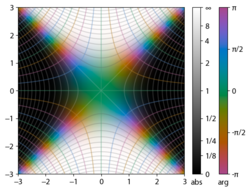
The error function is an odd function. This directly results from the fact that the integrand e − t 2 {\displaystyle e^{-t^{2}}} is an even function (since the antiderivative of an even function which is zero at the origin is an odd function, and vice versa).
Since the error function is an entire function which maps real numbers to real numbers, for any complex number z {\displaystyle z},
erf ( z ¯ ) = erf ( z ) ¯ {\displaystyle \operatorname {erf} ({\bar {z}})={\overline {\operatorname {erf} (z)}}}
where z ¯ {\displaystyle {\bar {z}}} denotes the complex conjugate of z {\displaystyle z}.
The error function at ∞ {\displaystyle \infty } is exactly 1 {\displaystyle 1} (see Gaussian integral). At the real axis, erf ( z ) {\displaystyle \operatorname {erf} (z)} approaches 1 {\displaystyle 1} at z → ∞ {\displaystyle z\to \infty } and − 1 {\displaystyle -1} at z → − ∞ {\displaystyle z\to -\infty }. At the imaginary axis, it tends to ± i ∞ {\displaystyle \pm i\infty }.
Taylor series
The error function is an entire function; it has no singularities (except at infinity) and its Taylor expansion always converges. For x ≫ 1 {\displaystyle x\gg 1}, however, cancellation of leading terms makes the Taylor expansion impractical.
The defining integral cannot be evaluated in closed form in terms of elementary functions (see Liouville's theorem), but by expanding the integrand e − z 2 {\displaystyle e^{-z^{2}}} into its Maclaurin series, integrating term by term, and using the fact that erf ( 0 ) = 0 {\displaystyle \operatorname {erf} (0)=0}, one obtains the error function's Maclaurin series as: erf ( z ) = 2 π ∑ n = 0 ∞ ( − 1 ) n z 2 n + 1 n ! ( 2 n + 1 ) = 2 π ( z − z 3 3 + z 5 10 − z 7 42 + z 9 216 − ⋯ ) {\displaystyle {\begin{aligned}\operatorname {erf} (z)&={\frac {2}{\sqrt {\pi }}}\sum _{n=0}^{\infty }{\frac {(-1)^{n}z^{2n+1}}{n!(2n+1)}}\\[6pt]&={\frac {2}{\sqrt {\pi }}}\left(z-{\frac {z^{3}}{3}}+{\frac {z^{5}}{10}}-{\frac {z^{7}}{42}}+{\frac {z^{9}}{216}}-\cdots \right)\end{aligned}}} which holds for every complex number z {\displaystyle z}. The denominator terms form sequence A007680 in the OEIS. This is a special case of Kummer's function:
erf ( z ) = 2 z π 1 F 1 ( 1 2 , 3 2 , − z 2 ) . {\displaystyle \operatorname {erf} (z)={\frac {2z}{\sqrt {\pi }}}\,{}_{1}F_{1}{\bigg (}{\frac {1}{2}},{\frac {3}{2}},-z^{2}{\bigg )}.}
For iterative calculation of the above series, the following alternative formulation may be useful: erf ( z ) = 2 π ∑ n = 0 ∞ ( z ∏ k = 1 n − ( 2 k − 1 ) z 2 k ( 2 k + 1 ) ) = 2 π ∑ n = 0 ∞ z 2 n + 1 ∏ k = 1 n − z 2 k , {\displaystyle {\begin{aligned}\operatorname {erf} (z)&={\frac {2}{\sqrt {\pi }}}\sum _{n=0}^{\infty }\left(z\prod _{k=1}^{n}{\frac {-(2k-1)z^{2}}{k(2k+1)}}\right)\\[6pt]&={\frac {2}{\sqrt {\pi }}}\sum _{n=0}^{\infty }{\frac {z}{2n+1}}\prod _{k=1}^{n}{\frac {-z^{2}}{k}},\end{aligned}}} because
− ( 2 k − 1 ) z 2 k ( 2 k + 1 ) {\displaystyle {\frac {-(2k-1)z^{2}}{k(2k+1)}}}
expresses the multiplier to turn the k {\displaystyle k}-th term into the ( k + 1 ) {\displaystyle (k+1)}-th term (considering z {\displaystyle z} as the first term).
The imaginary error function has a similar Maclaurin series: erfi ( z ) = 2 π ∑ n = 0 ∞ z 2 n + 1 n ! ( 2 n + 1 ) = 2 π ( z + z 3 3 + z 5 10 + z 7 42 + z 9 216 + ⋯ ) {\displaystyle {\begin{aligned}\operatorname {erfi} (z)&={\frac {2}{\sqrt {\pi }}}\sum _{n=0}^{\infty }{\frac {z^{2n+1}}{n!(2n+1)}}\\[6pt]&={\frac {2}{\sqrt {\pi }}}\left(z+{\frac {z^{3}}{3}}+{\frac {z^{5}}{10}}+{\frac {z^{7}}{42}}+{\frac {z^{9}}{216}}+\cdots \right)\end{aligned}}} which holds for every complex number z {\displaystyle z}.
Derivative and integral
The derivative of the error function follows immediately from its definition: d d z erf ( z ) = 2 π e − z 2 . {\displaystyle {\frac {d}{dz}}\operatorname {erf} (z)={\frac {2}{\sqrt {\pi }}}e^{-z^{2}}.} From this, the derivative of the imaginary error function is also immediate: d d z erfi ( z ) = 2 π e z 2 . {\displaystyle {\frac {d}{dz}}\operatorname {erfi} (z)={\frac {2}{\sqrt {\pi }}}e^{z^{2}}.}Higher order derivatives are given by erf ( k ) ( z ) = 2 ( − 1 ) k − 1 π H k − 1 ( z ) e − z 2 = 2 π d k − 1 d z k − 1 ( e − z 2 ) , {\displaystyle \operatorname {erf} ^{(k)}(z)={\frac {2(-1)^{k-1}}{\sqrt {\pi }}}{\mathit {H}}_{k-1}(z)e^{-z^{2}}={\frac {2}{\sqrt {\pi }}}{\frac {d^{k-1}}{dz^{k-1}}}{\big (}e^{-z^{2}}{\big )},} where the H k {\displaystyle H_{k}} are the physicists' Hermite polynomials.
An antiderivative of the error function, obtainable by integration by parts, is ∫ erf ( z ) d z = z erf ( z ) + e − z 2 π + C . {\displaystyle \int \operatorname {erf} (z)dz=z\operatorname {erf} (z)+{\frac {e^{-z^{2}}}{\sqrt {\pi }}}+C.} An antiderivative of the imaginary error function, also obtainable by integration by parts, is ∫ erfi ( z ) d z = z erfi ( z ) − e z 2 π + C . {\displaystyle \int \operatorname {erfi} (z)dz=z\operatorname {erfi} (z)-{\frac {e^{z^{2}}}{\sqrt {\pi }}}+C.}
Bürmann series
An expansion which converges more rapidly for all real values of x {\displaystyle x} than a Taylor expansion is obtained by using Bürmann's theorem: erf ( x ) = 2 π sgn ( x ) ⋅ 1 − e − x 2 ( 1 − 1 12 ( 1 − e − x 2 ) − 7 480 ( 1 − e − x 2 ) 2 − 5 896 ( 1 − e − x 2 ) 3 − ⋯ ) = 2 π sgn ( x ) ⋅ 1 − e − x 2 ( π 2 + ∑ k = 1 ∞ c k e − k x 2 ) {\displaystyle {\begin{aligned}\operatorname {erf} (x)&={\frac {2}{\sqrt {\pi }}}\operatorname {sgn}(x)\cdot {\sqrt {1-e^{-x^{2}}}}\left(1-{\frac {1}{12}}\left(1-e^{-x^{2}}\right)-{\frac {7}{480}}\left(1-e^{-x^{2}}\right)^{2}-{\frac {5}{896}}\left(1-e^{-x^{2}}\right)^{3}-\cdots \right)\\[10pt]&={\frac {2}{\sqrt {\pi }}}\operatorname {sgn}(x)\cdot {\sqrt {1-e^{-x^{2}}}}\left({\frac {\sqrt {\pi }}{2}}+\sum _{k=1}^{\infty }c_{k}e^{-kx^{2}}\right)\end{aligned}}} where sgn {\displaystyle \operatorname {sgn} } is the sign function. By keeping only the first two coefficients and choosing c 1 = 31 / 200 {\displaystyle c_{1}=31/200} and c 2 = − 341 / 8000 {\displaystyle c_{2}=-341/8000}, the resulting approximation shows its largest relative error at x = ± 1.40587 {\displaystyle x=\pm 1.40587}, where it is less than 0.0034361 {\displaystyle 0.0034361}: erf ( x ) ≈ 2 π sgn ( x ) ⋅ 1 − e − x 2 ( π 2 + 31 200 e − x 2 − 341 8000 e − 2 x 2 ) . {\displaystyle \operatorname {erf} (x)\approx {\frac {2}{\sqrt {\pi }}}\operatorname {sgn}(x)\cdot {\sqrt {1-e^{-x^{2}}}}\left({\frac {\sqrt {\pi }}{2}}+{\frac {31}{200}}e^{-x^{2}}-{\frac {341}{8000}}e^{-2x^{2}}\right).}
Inverse functions

Given a complex number z {\displaystyle z}, there is not a unique complex number w {\displaystyle w} satisfying erf ( w ) = z {\displaystyle \operatorname {erf} (w)=z}, so a true inverse function would be multivalued. However, for − 1 < x < 1 {\displaystyle -1<x<1}, there is a unique real number denoted erf − 1 ( x ) {\displaystyle \operatorname {erf} ^{-1}(x)} satisfying
erf ( erf − 1 ( x ) ) = x . {\displaystyle \operatorname {erf} \left(\operatorname {erf} ^{-1}(x)\right)=x.}
The inverse error function is usually defined with domain ( − 1 , 1 ) {\displaystyle (-1,1)}, and it is restricted to this domain in many computer algebra systems. However, it can be extended to the disk | z | < 1 {\displaystyle |z|<1} of the complex plane, using the Maclaurin series erf − 1 ( z ) = ∑ k = 0 ∞ c k 2 k + 1 ( π 2 z ) 2 k + 1 , {\displaystyle \operatorname {erf} ^{-1}(z)=\sum _{k=0}^{\infty }{\frac {c_{k}}{2k+1}}\left({\frac {\sqrt {\pi }}{2}}z\right)^{2k+1},} where c 0 = 1 {\displaystyle c_{0}=1} and c k = ∑ m = 0 k − 1 c m c k − 1 − m ( m + 1 ) ( 2 m + 1 ) = { 1 , 1 , 7 6 , 127 90 , 4369 2520 , 34807 16200 , … } . {\displaystyle {\begin{aligned}c_{k}&=\sum _{m=0}^{k-1}{\frac {c_{m}c_{k-1-m}}{(m+1)(2m+1)}}\\[1ex]&=\left\{1,1,{\frac {7}{6}},{\frac {127}{90}},{\frac {4369}{2520}},{\frac {34807}{16200}},\ldots \right\}.\end{aligned}}}
So we have the series expansion (common factors have been canceled from numerators and denominators):
erf − 1 ( z ) = π 2 ( z + π 12 z 3 + 7 π 2 480 z 5 + 127 π 3 40320 z 7 + 4369 π 4 5806080 z 9 + 34807 π 5 182476800 z 11 + ⋯ ) . {\displaystyle \operatorname {erf} ^{-1}(z)={\frac {\sqrt {\pi }}{2}}\left(z+{\frac {\pi }{12}}z^{3}+{\frac {7\pi ^{2}}{480}}z^{5}+{\frac {127\pi ^{3}}{40320}}z^{7}+{\frac {4369\pi ^{4}}{5806080}}z^{9}+{\frac {34807\pi ^{5}}{182476800}}z^{11}+\cdots \right).}
(After cancellation the numerator and denominator values in (sequenceA092676in theOEIS) and (sequenceA092677in theOEIS) respectively; without cancellation the numerator terms are values in (sequenceA002067in theOEIS).) The error function's value at ± ∞ {\displaystyle \pm \infty } is equal to ± 1 {\displaystyle \pm 1}.
For | z | < 1 {\displaystyle |z|<1}, we have erf ( erf − 1 ( z ) ) = z {\displaystyle \operatorname {erf} (\operatorname {erf} ^{-1}(z))=z}.
The inverse complementary error function is defined as erfc − 1 ( 1 − z ) = erf − 1 ( z ) . {\displaystyle \operatorname {erfc} ^{-1}(1-z)=\operatorname {erf} ^{-1}(z).} For real x {\displaystyle x}, there is a unique real number erfi − 1 ( x ) {\displaystyle \operatorname {erfi} ^{-1}(x)} satisfying erfi ( erfi − 1 ( x ) ) = x {\displaystyle \operatorname {erfi} (\operatorname {erfi} ^{-1}(x))=x}. The inverse imaginary error function is defined as erfi − 1 ( x ) {\displaystyle \operatorname {erfi} ^{-1}(x)}.
For any real x {\displaystyle x}, Newton's method can be used to compute erfi − 1 ( x ) {\displaystyle \operatorname {erfi} ^{-1}(x)}, and for − 1 ≤ x ≤ 1 {\displaystyle -1\leq x\leq 1}, the following Maclaurin series converges:
erfi − 1 ( z ) = ∑ k = 0 ∞ ( − 1 ) k c k 2 k + 1 ( π 2 z ) 2 k + 1 , {\displaystyle \operatorname {erfi} ^{-1}(z)=\sum _{k=0}^{\infty }{\frac {(-1)^{k}c_{k}}{2k+1}}\left({\frac {\sqrt {\pi }}{2}}z\right)^{2k+1},}
where c k {\displaystyle c_{k}} is defined as above.
Asymptotic expansion
A useful asymptotic expansion of the complementary error function (and therefore also of the error function) for large real x {\displaystyle x} is erfc ( x ) = e − x 2 x π ( 1 + ∑ n = 1 ∞ ( − 1 ) n 1 ⋅ 3 ⋅ 5 ⋯ ( 2 n − 1 ) ( 2 x 2 ) n ) = e − x 2 x π ∑ n = 0 ∞ ( − 1 ) n ( 2 n − 1 ) ! ! ( 2 x 2 ) n , {\displaystyle {\begin{aligned}\operatorname {erfc} (x)&={\frac {e^{-x^{2}}}{x{\sqrt {\pi }}}}\left(1+\sum _{n=1}^{\infty }(-1)^{n}{\frac {1\cdot 3\cdot 5\cdots (2n-1)}{\left(2x^{2}\right)^{n}}}\right)\\[6pt]&={\frac {e^{-x^{2}}}{x{\sqrt {\pi }}}}\sum _{n=0}^{\infty }(-1)^{n}{\frac {(2n-1)!!}{\left(2x^{2}\right)^{n}}},\end{aligned}}} where ( 2 n − 1 ) ! ! {\displaystyle (2n-1)!!} is the double factorial of 2 n − 1 {\displaystyle 2n-1}, i.e. the product of all odd numbers up to 2 n − 1 {\displaystyle 2n-1}. This series diverges for every finite x {\displaystyle x}, and its meaning as asymptotic expansion is that for any integer N ≥ 1 {\displaystyle N\geq 1} one has
erfc ( x ) = e − x 2 x π ∑ n = 0 N − 1 ( − 1 ) n ( 2 n − 1 ) ! ! ( 2 x 2 ) n + R N ( x ) , {\displaystyle \operatorname {erfc} (x)={\frac {e^{-x^{2}}}{x{\sqrt {\pi }}}}\sum _{n=0}^{N-1}(-1)^{n}{\frac {(2n-1)!!}{\left(2x^{2}\right)^{n}}}+R_{N}(x),}
where the remainder is
R N ( x ) := ( − 1 ) N ( 2 N − 1 ) ! ! π ⋅ 2 N − 1 ∫ x ∞ t − 2 N e − t 2 d t , {\displaystyle R_{N}(x):={\frac {(-1)^{N}\,(2N-1)!!}{{\sqrt {\pi }}\cdot 2^{N-1}}}\int _{x}^{\infty }t^{-2N}e^{-t^{2}}\,dt,}
which follows easily by induction, writing
e − t 2 = − 1 2 t d d t e − t 2 {\displaystyle e^{-t^{2}}=-{\frac {1}{2t}}\,{\frac {d}{dt}}e^{-t^{2}}}
and integrating by parts. The asymptotic behavior of the remainder term is
R N ( x ) = O ( x − ( 1 + 2 N ) e − x 2 ) {\displaystyle R_{N}(x)=O{\Big (}x^{-(1+2N)}e^{-x^{2}}{\Big )}}
as x → ∞ {\displaystyle x\to \infty }. This can be found by
R N ( x ) ∝ ∫ x ∞ t − 2 N e − t 2 d t = e − x 2 ∫ 0 ∞ ( t + x ) − 2 N e − t 2 − 2 t x d t ≤ e − x 2 ∫ 0 ∞ x − 2 N e − 2 t x d t ∝ x − ( 1 + 2 N ) e − x 2 . {\displaystyle R_{N}(x)\propto \int _{x}^{\infty }t^{-2N}e^{-t^{2}}\,dt=e^{-x^{2}}\int _{0}^{\infty }(t+x)^{-2N}e^{-t^{2}-2tx}\,dt\leq e^{-x^{2}}\int _{0}^{\infty }x^{-2N}e^{-2tx}\,dt\propto x^{-(1+2N)}e^{-x^{2}}.}
For large enough values of x {\displaystyle x}, only the first few terms of this asymptotic expansion are needed to obtain a good approximation of erfc ( x ) {\displaystyle \operatorname {erfc} (x)} (while for not too large values of x {\displaystyle x}, the above Taylor expansion at 0 provides a very fast convergence).
Continued fraction expansion
A continued fraction expansion of the complementary error function was found by Laplace: erfc ( z ) = z π e − z 2 1 z 2 + a 1 1 + a 2 z 2 + a 3 1 + ⋯ {\displaystyle \operatorname {erfc} (z)={\frac {z}{\sqrt {\pi }}}e^{-z^{2}}{\cfrac {1}{z^{2}+{\cfrac {a_{1}}{1+{\cfrac {a_{2}}{z^{2}+{\cfrac {a_{3}}{1+\dotsb }}}}}}}}} where a m = m 2 {\displaystyle a_{m}={\frac {m}{2}}}.
Factorial series
The inverse factorial series
erfc ( z ) = e − z 2 π z ∑ n = 0 ∞ ( − 1 ) n Q n ( z 2 + 1 ) ( n ) = e − z 2 π z [ 1 − 1 2 1 ( z 2 + 1 ) + 1 4 1 ( z 2 + 1 ) ( z 2 + 2 ) − ⋯ ] {\displaystyle {\begin{aligned}\operatorname {erfc} (z)&={\frac {e^{-z^{2}}}{{\sqrt {\pi }}\,z}}\sum _{n=0}^{\infty }{\frac {\left(-1\right)^{n}Q_{n}}{{\left(z^{2}+1\right)}^{(n)}}}\\[1ex]&={\frac {e^{-z^{2}}}{{\sqrt {\pi }}\,z}}\left[1-{\frac {1}{2}}{\frac {1}{(z^{2}+1)}}+{\frac {1}{4}}{\frac {1}{\left(z^{2}+1\right)\left(z^{2}+2\right)}}-\cdots \right]\end{aligned}}}
converges for Re ( z 2 ) > 0 {\displaystyle \operatorname {Re} (z^{2})>0}. Here
Q n = 1 π ∫ 0 ∞ τ ( τ − 1 ) ⋯ ( τ − n + 1 ) τ − 1 2 e − τ d τ = ∑ k = 0 n s ( n , k ) ( 1 2 ) ( k ) = ∑ k = 0 n s ( n , k ) ( 2 k − 1 ) ! ! 2 k {\displaystyle {\begin{aligned}Q_{n}&={\frac {1}{\sqrt {\pi }}}\int _{0}^{\infty }\tau (\tau -1)\cdots (\tau -n+1)\tau ^{-{\frac {1}{2}}}e^{-\tau }\,d\tau \\[1ex]&=\sum _{k=0}^{n}s(n,k)\left({\frac {1}{2}}\right)^{(k)}=\sum _{k=0}^{n}s(n,k){\frac {(2k-1)!!}{2^{k}}}\end{aligned}}}
where z ( n ) {\displaystyle z^{(n)}} denotes the rising factorial, and s ( n , k ) {\displaystyle s(n,k)} denotes a signed Stirling number of the first kind. The Taylor series can be written in terms of the double factorial:
erf ( z ) = 2 π ∑ n = 0 ∞ ( − 2 ) n ( 2 n − 1 ) ! ! ( 2 n + 1 ) ! z 2 n + 1 . {\displaystyle \operatorname {erf} (z)={\frac {2}{\sqrt {\pi }}}\sum _{n=0}^{\infty }{\frac {(-2)^{n}(2n-1)!!}{(2n+1)!}}z^{2n+1}.}
Bounds and numerical approximations
Approximation with elementary functions
Abramowitz and Stegun give several approximations of varying accuracy (equations 7.1.25–28). This allows one to choose the fastest approximation suitable for a given application. In order of increasing accuracy, they are: erf ( x ) ≈ 1 − 1 ( 1 + a 1 x + a 2 x 2 + a 3 x 3 + a 4 x 4 ) 4 , x ≥ 0 {\displaystyle \operatorname {erf} (x)\approx 1-{\frac {1}{\left(1+a_{1}x+a_{2}x^{2}+a_{3}x^{3}+a_{4}x^{4}\right)^{4}}},\qquad x\geq 0} (maximum error: 5×10⁻⁴)
where a1 = 0.278393, a2 = 0.230389, a3 = 0.000972, a4 = 0.078108
erf ( x ) ≈ 1 − ( a 1 t + a 2 t 2 + a 3 t 3 ) e − x 2 , t = 1 1 + p x , x ≥ 0 {\displaystyle \operatorname {erf} (x)\approx 1-\left(a_{1}t+a_{2}t^{2}+a_{3}t^{3}\right)e^{-x^{2}},\quad t={\frac {1}{1+px}},\qquad x\geq 0} (maximum error: 2.5×10⁻⁵)
where p = 0.47047, a1 = 0.3480242, a2 = −0.0958798, a3 = 0.7478556
erf ( x ) ≈ 1 − 1 ( 1 + a 1 x + a 2 x 2 + ⋯ + a 6 x 6 ) 16 , x ≥ 0 {\displaystyle \operatorname {erf} (x)\approx 1-{\frac {1}{\left(1+a_{1}x+a_{2}x^{2}+\cdots +a_{6}x^{6}\right)^{16}}},\qquad x\geq 0} (maximum error: 3×10⁻⁷)
where a1 = 0.0705230784, a2 = 0.0422820123, a3 = 0.0092705272, a4 = 0.0001520143, a5 = 0.0002765672, a6 = 0.0000430638
erf ( x ) ≈ 1 − ( a 1 t + a 2 t 2 + ⋯ + a 5 t 5 ) e − x 2 , t = 1 1 + p x {\displaystyle \operatorname {erf} (x)\approx 1-\left(a_{1}t+a_{2}t^{2}+\cdots +a_{5}t^{5}\right)e^{-x^{2}},\quad t={\frac {1}{1+px}}} (maximum error: 1.5×10⁻⁷)
where p = 0.3275911, a1 = 0.254829592, a2 = −0.284496736, a3 = 1.421413741, a4 = −1.453152027, a5 = 1.061405429
One can improve the accuracy of the A&S approximation by extending it with three extra parameters, erf ( x ) ≈ 1 − ( a 1 t + a 2 t 2 + ⋯ + a 5 t 5 + a 6 t 6 + a 7 t 7 ) e − x 2 , t = 1 1 + p 1 x + p 2 x 2 {\displaystyle \operatorname {erf} (x)\approx 1-\left(a_{1}t+a_{2}t^{2}+\cdots +a_{5}t^{5}+a_{6}t^{6}+a_{7}t^{7}\right)e^{-x^{2}},\quad t={\frac {1}{1+p_{1}x+p_{2}x^{2}}}} where p1 = 0.406742016006509, p2 = 0.0072279182302319, a1 = 0.316879890481381, a2 = -0.138329314150635, a3 = 1.08680830347054, a4 = -1.11694155120396, a5 = 1.20644903073232, a6 = -0.393127715207728, a7 = 0.0382613542530727. The maximum error of this approximation is about 2×10⁻⁹. The parameters are obtained by fitting the extended approximation to the accurate values of the error function using the following Python code.
| Python code to fit extended A&S approximation |
|---|
| importnumpyasnp frommathimport erf, exp, sqrt fromscipy.optimizeimport least_squares # # Extended A&S approximation: # erf(x) ≈ 1 − t * exp(−x^2) * (a1 + a2*t + a3*t^2 + ... + a7*t^6) # where now # t = 1 / (1 + p1*x + p2*x^2) # We fit parameters p1, p2, a1..a7 over x in [0, 10]. # defapprox_erf(params, x): p1 = params[0] p2 = params[1] a = params[2:] t = 1.0 / (1.0 + p1 * x + p2 * x * x) poly = np.zeros_like(x) tt = np.ones_like(x) # t^0 # polynomial: a1*t^0 + a2*t^1 + ... + a7*t^6 for ak in a: poly += ak * tt tt *= t return 1.0 - t * np.exp(-x * x) * poly defresiduals(params, xs, ys): return approx_erf(params, xs) - ys # # Prepare data for fitting # N = 300 xmin = 0 xmax = 10 xs = np.linspace(xmin, xmax, N) ys = np.array([erf(x) for x in xs], dtype=float) # # Initial guess for parameters # Start from original A&S values and extend them conservatively # p1_0 = 0.3275911 # original A&S p p2_0 = 0.0 # new denominator parameter # original A&S 5 coefficients, add two => 7 in total a0 = [ 0.254829592, -0.284496736, 1.421413741, -1.453152027, 1.061405429, 0.0, # new term 0.0, # another new term ] params0 = np.array([p1_0, p2_0] + a0, dtype=float) # # Fit using nonlinear least squares (Levenberg–Marquardt) # result = least_squares( residuals, params0, args=(xs, ys), xtol=1e-14, ftol=1e-14, gtol=1e-14, max_nfev=5000 ) params = result.x p1_fit = params[0] p2_fit = params[1] a_fit = params[2:] # # Print fitted parameters # print("\nFitted parameters:") print(f"p1 ={p1_fit:.15g},") print(f"p2 ={p2_fit:.15g},") for i, ai in enumerate(a_fit, 1): print(f"a{i}={ai:.15g},") # # Evaluate approximation error # approx_vals = approx_erf(params, xs) abs_err = np.abs(approx_vals - ys) print(f"\nMaximum absolute error on [{xmin},{xmax}]:", np.max(abs_err)) print("RMS error:", np.sqrt(np.mean(abs_err**2))) print("Done.") |
All of these approximations are valid for x ≥ 0. To use these approximations for negative x, use the fact that erf(x) is an odd function, so erf(x) = −erf(−x).
Exponential bounds and a pure exponential approximation for the complementary error function are given by erfc ( x ) ≤ 1 2 e − 2 x 2 + 1 2 e − x 2 ≤ e − x 2 , x > 0 erfc ( x ) ≈ 1 6 e − x 2 + 1 2 e − 4 3 x 2 , x > 0. {\displaystyle {\begin{aligned}\operatorname {erfc} (x)&\leq {\frac {1}{2}}e^{-2x^{2}}+{\frac {1}{2}}e^{-x^{2}}\leq e^{-x^{2}},&&x>0\\[1.5ex]\operatorname {erfc} (x)&\approx {\frac {1}{6}}e^{-x^{2}}+{\frac {1}{2}}e^{-{\frac {4}{3}}x^{2}},&&x>0.\end{aligned}}}
The above have been generalized to sums of N exponentials with increasing accuracy in terms of N so that erfc(x) can be accurately approximated or bounded by 2Q̃(√2x), where Q ~ ( x ) = ∑ n = 1 N a n e − b n x 2 . {\displaystyle {\tilde {Q}}(x)=\sum _{n=1}^{N}a_{n}e^{-b_{n}x^{2}}.} In particular, there is a systematic methodology to solve the numerical coefficients {(an,bn)}N n = 1 that yield a minimax approximation or bound for the closely related Q-function: Q(x) ≈ Q̃(x), Q(x) ≤ Q̃(x), or Q(x) ≥ Q̃(x) for x ≥ 0. The coefficients {(an,bn)}N n = 1 for many variations of the exponential approximations and bounds up to N = 25 have been released to open access as a comprehensive dataset.
A tight approximation of the complementary error function for x ∈ [0,∞) is given by Karagiannidis & Lioumpas (2007), who showed for the appropriate choice of parameters {A,B} that erfc ( x ) ≈ ( 1 − e − A x ) e − x 2 B π x . {\displaystyle \operatorname {erfc} (x)\approx {\frac {\left(1-e^{-Ax}\right)e^{-x^{2}}}{B{\sqrt {\pi }}x}}.} They determined {A,B} = {1.98,1.135}, which gave a good approximation[which?] for all x ≥ 0. Alternative coefficients are also available for tailoring accuracy for a specific application or transforming the expression into a tight bound.
A single-term lower bound is erfc ( x ) ≥ 2 e π β − 1 β e − β x 2 , x ≥ 0 , β > 1 , {\displaystyle \operatorname {erfc} (x)\geq {\sqrt {\frac {2e}{\pi }}}{\frac {\sqrt {\beta -1}}{\beta }}e^{-\beta x^{2}},\qquad x\geq 0,\quad \beta >1,} where the parameter β can be picked to minimize error on the desired interval of approximation.
Another approximation is given by Sergei Winitzki using his "global Padé approximations": erf ( x ) ≈ sgn x ⋅ 1 − exp ( − x 2 4 π + a x 2 1 + a x 2 ) {\displaystyle \operatorname {erf} (x)\approx \operatorname {sgn} x\cdot {\sqrt {1-\exp \left(-x^{2}{\frac {{\frac {4}{\pi }}+ax^{2}}{1+ax^{2}}}\right)}}} where a = 8 ( π − 3 ) 3 π ( 4 − π ) ≈ 0.140012. {\displaystyle a={\frac {8(\pi -3)}{3\pi (4-\pi )}}\approx 0.140012.} This is designed to be very accurate in the neighborhoods of 0 and infinity, and the relative error is less than 0.00035 for all real x. Using the alternate value a ≈ 0.147 reduces the maximum relative error to about 0.00013.
The extended "global Pade" approximation, erf ( x ) ≈ sgn x ⋅ 1 − exp ( − x 2 4 + 0.880877880079853 x 2 + 0.144026670907584 x 4 + 0.0077581300270021 x 6 π + 0.786235558186528 x 2 + 0.128368576906837 x 4 + 0.00773380006014367 x 6 ) , {\displaystyle \operatorname {erf} (x)\approx \operatorname {sgn} x\cdot {\sqrt {1-\exp \left(-x^{2}{\frac {4+0.880877880079853x^{2}+0.144026670907584x^{4}+0.0077581300270021x^{6}}{\pi +0.786235558186528x^{2}+0.128368576906837x^{4}+0.00773380006014367x^{6}}}\right)}}\,,} provides a maximum error of about 2×10⁻⁹, as demonstrated by the following Python script.
| Python script to fit extended "global Pade" approximation |
|---|
| importnumpy,math fromscipy.optimizeimport least_squares # approximation to erf(x) defapprox_erf(p,x): frac=(4+p[0]*x**2+p[1]*x**4+p[2]*x**6)/( math.pi+p[3]*x**2+p[4]*x**4+p[5]*x**6) return numpy.sign(x)*numpy.sqrt( 1-numpy.exp(-x*x*frac)) defresiduals(params, xs, ys): return approx_erf(params, xs) - ys # data for fitting N = 200 xmin = 0 xmax = 9 xs = numpy.linspace(xmin, xmax, N) ys = numpy.array([math.erf(x) for x in xs], dtype=float) params0 = numpy.array([0.9,0.1,0.008,0.8,0.1,0.008], dtype=float) # fitting result = least_squares( residuals, params0, args=(xs, ys), xtol=1e-14, ftol=1e-14, gtol=1e-14, max_nfev=5000 ) params = result.x # print out fitted parameters print("\nFitted parameters:") for i, pi in enumerate(params, 0): print(f"p{i}={pi:.15g},") # evaluate approximation error approx_vals = approx_erf(params, xs) abs_err = numpy.abs(approx_vals - ys) print(f"\nMaximum absolute error on [{xmin},{xmax}]:", numpy.max(abs_err)) print("RMS error:", numpy.sqrt(numpy.mean(abs_err**2))) print("Done.") |
Winitzki's approximation can be inverted to obtain an approximation for the inverse error function: erf − 1 ( x ) ≈ sgn x ⋅ ( 2 π a + ln ( 1 − x 2 ) 2 ) 2 − ln ( 1 − x 2 ) a − ( 2 π a + ln ( 1 − x 2 ) 2 ) . {\displaystyle \operatorname {erf} ^{-1}(x)\approx \operatorname {sgn} x\cdot {\sqrt {{\sqrt {\left({\frac {2}{\pi a}}+{\frac {\ln \left(1-x^{2}\right)}{2}}\right)^{2}-{\frac {\ln \left(1-x^{2}\right)}{a}}}}-\left({\frac {2}{\pi a}}+{\frac {\ln \left(1-x^{2}\right)}{2}}\right)}}.}
An approximation with a maximal error of 1.2×10⁻⁷ for any real argument is: erf ( x ) = { 1 − τ , x ≥ 0 τ − 1 , x < 0 τ = t ⋅ exp ( − x 2 − 1.26551223 + 1.00002368 t + 0.37409196 t 2 + 0.09678418 t 3 − 0.18628806 t 4 + 0.27886807 t 5 − 1.13520398 t 6 + 1.48851587 t 7 − 0.82215223 t 8 + 0.17087277 t 9 ) t = 1 1 + 1 2 | x | {\displaystyle {\begin{aligned}\operatorname {erf} (x)&={\begin{cases}1-\tau ,&x\geq 0\\\tau -1,&x<0\end{cases}}\\\tau &=t\cdot \exp \left(-x^{2}-1.26551223+1.00002368t+0.37409196t^{2}+0.09678418t^{3}-0.18628806t^{4}\right.\\&\left.\qquad \qquad \qquad +0.27886807t^{5}-1.13520398t^{6}+1.48851587t^{7}-0.82215223t^{8}+0.17087277t^{9}\right)\\t&={\frac {1}{1+{\frac {1}{2}}|x|}}\end{aligned}}}
An approximation of erfc {\displaystyle \operatorname {erfc} } with a maximum relative error less than 2 − 53 {\displaystyle 2^{-53}} ( ≈ 1.1 × 10 − 16 ) {\displaystyle \left(\approx 1.1\times 10^{-16}\right)} in absolute value is: for x ≥ 0 {\displaystyle x\geq 0}, erfc ( x ) = ( 0.56418958354775629 x + 2.06955023132914151 ) ( x 2 + 2.71078540045147805 x + 5.80755613130301624 x 2 + 3.47954057099518960 x + 12.06166887286239555 ) ( x 2 + 3.47469513777439592 x + 12.07402036406381411 x 2 + 3.72068443960225092 x + 8.44319781003968454 ) ( x 2 + 4.00561509202259545 x + 9.30596659485887898 x 2 + 3.90225704029924078 x + 6.36161630953880464 ) ( x 2 + 5.16722705817812584 x + 9.12661617673673262 x 2 + 4.03296893109262491 x + 5.13578530585681539 ) ( x 2 + 5.95908795446633271 x + 9.19435612886969243 x 2 + 4.11240942957450885 x + 4.48640329523408675 ) e − x 2 {\displaystyle {\begin{aligned}\operatorname {erfc} \left(x\right)&=\left({\frac {0.56418958354775629}{x+2.06955023132914151}}\right)\left({\frac {x^{2}+2.71078540045147805x+5.80755613130301624}{x^{2}+3.47954057099518960x+12.06166887286239555}}\right)\\&\left({\frac {x^{2}+3.47469513777439592x+12.07402036406381411}{x^{2}+3.72068443960225092x+8.44319781003968454}}\right)\left({\frac {x^{2}+4.00561509202259545x+9.30596659485887898}{x^{2}+3.90225704029924078x+6.36161630953880464}}\right)\\&\left({\frac {x^{2}+5.16722705817812584x+9.12661617673673262}{x^{2}+4.03296893109262491x+5.13578530585681539}}\right)\left({\frac {x^{2}+5.95908795446633271x+9.19435612886969243}{x^{2}+4.11240942957450885x+4.48640329523408675}}\right)e^{-x^{2}}\\\end{aligned}}} and for x < 0 {\displaystyle x<0} erfc ( x ) = 2 − erfc ( − x ) {\displaystyle \operatorname {erfc} \left(x\right)=2-\operatorname {erfc} \left(-x\right)}
A simple approximation for real-valued arguments can be done through hyperbolic functions: erf ( x ) ≈ z ( x ) = tanh ( 2 π ( x + 11 123 x 3 ) ) {\displaystyle \operatorname {erf} \left(x\right)\approx z(x)=\tanh \left({\frac {2}{\sqrt {\pi }}}\left(x+{\frac {11}{123}}x^{3}\right)\right)} which keeps the absolute difference | erf ( x ) − z ( x ) | < 0.000358 , ∀ x {\displaystyle \left|\operatorname {erf} \left(x\right)-z(x)\right|<0.000358,\,\forall x}.
Since the error function and the Gaussian Q-function are closely related through the identity erfc ( x ) = 2 Q ( 2 x ) {\displaystyle \operatorname {erfc} (x)=2Q({\sqrt {2}}x)} or equivalently Q ( x ) = 1 2 erfc ( x 2 ) {\displaystyle Q(x)={\frac {1}{2}}\operatorname {erfc} \left({\frac {x}{\sqrt {2}}}\right)}, bounds developed for the Q-function can be adapted to approximate the complementary error function. A pair of tight lower and upper bounds on the Gaussian Q-function for positive arguments x ∈ [ 0 , ∞ ) {\displaystyle x\in [0,\infty )} was introduced by Abreu (2012) based on a simple algebraic expression with only two exponential terms: x ≥ 0 1 2 erfc ( x 2 ) ≥ 1 12 e − x 2 + 1 2 π ( x + 1 ) e − x 2 / 2 ≤ 1 50 e − x 2 + 1 2 ( x + 1 ) e − x 2 / 2 1 25 e − 2 x 2 + 1 x + 1 e − x 2 ≥ erfc ( x ) ≥ 1 6 e − 2 x 2 + 1 2 2 π ( x + 1 ) e − x 2 {\displaystyle {\begin{aligned}x&\geq 0\\{\frac {1}{2}}\operatorname {erfc} \left({\frac {x}{\sqrt {2}}}\right)&\geq {\frac {1}{12}}e^{-x^{2}}+{\frac {1}{{\sqrt {2\pi }}(x+1)}}e^{-x^{2}/2}\\&\leq {\frac {1}{50}}e^{-x^{2}}+{\frac {1}{2(x+1)}}e^{-x^{2}/2}\\{\frac {1}{25}}e^{-2x^{2}}+{\frac {1}{x+1}}e^{-x^{2}}\geq \operatorname {erfc} (x)&\geq {\frac {1}{6}}e^{-2x^{2}}+{\frac {1}{2{\sqrt {2\pi }}(x+1)}}e^{-x^{2}}\end{aligned}}}
These bounds stem from a unified form Q B ( x ; a , b ) = exp ( − x 2 ) a + exp ( − x 2 / 2 ) b ( x + 1 ) , {\displaystyle Q_{\mathrm {B} }(x;a,b)={\frac {\exp(-x^{2})}{a}}+{\frac {\exp(-x^{2}/2)}{b(x+1)}},} where the parameters a {\displaystyle a} and b {\displaystyle b} are selected to ensure the bounding properties: for the lower bound, a L = 12 {\displaystyle a_{\mathrm {L} }=12} and b L = 2 π {\displaystyle b_{\mathrm {L} }={\sqrt {2\pi }}}, and for the upper bound, a U = 50 {\displaystyle a_{\mathrm {U} }=50} and b U = 2 {\displaystyle b_{\mathrm {U} }=2}. These expressions maintain simplicity and tightness, providing a practical trade-off between accuracy and ease of computation. They are particularly valuable in theoretical contexts, such as communication theory over fading channels, where both functions frequently appear. Additionally, the original Q-function bounds can be extended to Q n ( x ) {\displaystyle Q^{n}(x)} for positive integers n {\displaystyle n} via the binomial theorem, suggesting potential adaptability for powers of erfc ( x ) {\displaystyle \operatorname {erfc} (x)}, though this is less commonly required in error function applications.
Table of values
| x | erf(x) | 1 − erf(x) |
|---|---|---|
| 0 | 0 | 1 |
| 0.02 | 0.022564575 | 0.977435425 |
| 0.04 | 0.045111106 | 0.954888894 |
| 0.06 | 0.067621594 | 0.932378406 |
| 0.08 | 0.090078126 | 0.909921874 |
| 0.1 | 0.112462916 | 0.887537084 |
| 0.2 | 0.222702589 | 0.777297411 |
| 0.3 | 0.328626759 | 0.671373241 |
| 0.4 | 0.428392355 | 0.571607645 |
| 0.5 | 0.520499878 | 0.479500122 |
| 0.6 | 0.603856091 | 0.396143909 |
| 0.7 | 0.677801194 | 0.322198806 |
| 0.8 | 0.742100965 | 0.257899035 |
| 0.9 | 0.796908212 | 0.203091788 |
| 1 | 0.842700793 | 0.157299207 |
| 1.1 | 0.880205070 | 0.119794930 |
| 1.2 | 0.910313978 | 0.089686022 |
| 1.3 | 0.934007945 | 0.065992055 |
| 1.4 | 0.952285120 | 0.047714880 |
| 1.5 | 0.966105146 | 0.033894854 |
| 1.6 | 0.976348383 | 0.023651617 |
| 1.7 | 0.983790459 | 0.016209541 |
| 1.8 | 0.989090502 | 0.010909498 |
| 1.9 | 0.992790429 | 0.007209571 |
| 2 | 0.995322265 | 0.004677735 |
| 2.1 | 0.997020533 | 0.002979467 |
| 2.2 | 0.998137154 | 0.001862846 |
| 2.3 | 0.998856823 | 0.001143177 |
| 2.4 | 0.999311486 | 0.000688514 |
| 2.5 | 0.999593048 | 0.000406952 |
| 3 | 0.999977910 | 0.000022090 |
| 3.5 | 0.999999257 | 0.000000743 |
Related functions
Complementary error function

The complementary error function, denoted erfc, is defined as erfc ( x ) = 1 − erf ( x ) = 2 π ∫ x ∞ e − t 2 d t = e − x 2 erfcx ( x ) , {\displaystyle {\begin{aligned}\operatorname {erfc} (x)&=1-\operatorname {erf} (x)\\&={\frac {2}{\sqrt {\pi }}}\int _{x}^{\infty }e^{-t^{2}}\,dt\\&=e^{-x^{2}}\operatorname {erfcx} (x),\end{aligned}}} which also defines erfcx, the scaled complementary error function (which can be used instead of erfc to avoid arithmetic underflow). Another form of erfc x for x ≥ 0 is known as Craig's formula, after its discoverer: erfc ( x ∣ x ≥ 0 ) = 2 π ∫ 0 π 2 exp ( − x 2 sin 2 θ ) d θ . {\displaystyle \operatorname {erfc} (x\mid x\geq 0)={\frac {2}{\pi }}\int _{0}^{\frac {\pi }{2}}\exp \left(-{\frac {x^{2}}{\sin ^{2}\theta }}\right)\,d\theta .} This expression is valid only for positive values of x, but can be used in conjunction with erfc(x) = 2 − erfc(−x) to obtain erfc(x) for negative values. This form is advantageous in that the range of integration is fixed and finite. An extension of this expression for the erfc of the sum of two non-negative variables is erfc ( x + y ∣ x , y ≥ 0 ) = 2 π ∫ 0 π 2 exp ( − x 2 sin 2 θ − y 2 cos 2 θ ) d θ . {\displaystyle \operatorname {erfc} (x+y\mid x,y\geq 0)={\frac {2}{\pi }}\int _{0}^{\frac {\pi }{2}}\exp \left(-{\frac {x^{2}}{\sin ^{2}\theta }}-{\frac {y^{2}}{\cos ^{2}\theta }}\right)\,d\theta .}
Imaginary error function

The imaginary error function, denoted erfi, is defined as erfi ( x ) = − i erf ( i x ) = 2 π ∫ 0 x e t 2 d t = 2 π e x 2 D ( x ) , {\displaystyle {\begin{aligned}\operatorname {erfi} (x)&=-i\operatorname {erf} (ix)\\&={\frac {2}{\sqrt {\pi }}}\int _{0}^{x}e^{t^{2}}\,dt\\&={\frac {2}{\sqrt {\pi }}}e^{x^{2}}D(x),\end{aligned}}} where D(x) is the Dawson function (which can be used instead of erfi to avoid arithmetic overflow).
Despite the name "imaginary error function", erfi(x) is real when x is real.
When the error function is evaluated for arbitrary complex arguments z, the resulting complex error function is usually discussed in scaled form as the Faddeeva function: w ( z ) = e − z 2 erfc ( − i z ) = erfcx ( − i z ) . {\displaystyle w(z)=e^{-z^{2}}\operatorname {erfc} (-iz)=\operatorname {erfcx} (-iz).}
Cumulative distribution function

The error function is essentially identical to the standard normal cumulative distribution function, denoted Φ, also named norm(x) by some software languages[citation needed], as they differ only by scaling and translation. Indeed, Φ ( x ) = 1 2 π ∫ − ∞ x e − t 2 2 d t = 1 2 ( 1 + erf ( x 2 ) ) = 1 2 erfc ( − x 2 ) {\displaystyle {\begin{aligned}\Phi (x)&={\frac {1}{\sqrt {2\pi }}}\int _{-\infty }^{x}e^{\tfrac {-t^{2}}{2}}\,dt\\[6pt]&={\frac {1}{2}}\left(1+\operatorname {erf} \left({\frac {x}{\sqrt {2}}}\right)\right)\\[6pt]&={\frac {1}{2}}\operatorname {erfc} \left(-{\frac {x}{\sqrt {2}}}\right)\end{aligned}}} or rearranged for erf and erfc: erf ( x ) = 2 Φ ( x 2 ) − 1 erfc ( x ) = 2 Φ ( − x 2 ) = 2 ( 1 − Φ ( x 2 ) ) . {\displaystyle {\begin{aligned}\operatorname {erf} (x)&=2\Phi {\left(x{\sqrt {2}}\right)}-1\\[6pt]\operatorname {erfc} (x)&=2\Phi {\left(-x{\sqrt {2}}\right)}\\&=2\left(1-\Phi {\left(x{\sqrt {2}}\right)}\right).\end{aligned}}}
Consequently, the error function is also closely related to the Q-function, which is the tail probability of the standard normal distribution. The Q-function can be expressed in terms of the error function as Q ( x ) = 1 2 − 1 2 erf ( x 2 ) = 1 2 erfc ( x 2 ) . {\displaystyle {\begin{aligned}Q(x)&={\frac {1}{2}}-{\frac {1}{2}}\operatorname {erf} \left({\frac {x}{\sqrt {2}}}\right)\\&={\frac {1}{2}}\operatorname {erfc} \left({\frac {x}{\sqrt {2}}}\right).\end{aligned}}}
The inverse of Φ is known as the normal quantile function, or probit function and may be expressed in terms of the inverse error function as probit ( p ) = Φ − 1 ( p ) = 2 erf − 1 ( 2 p − 1 ) = − 2 erfc − 1 ( 2 p ) . {\displaystyle \operatorname {probit} (p)=\Phi ^{-1}(p)={\sqrt {2}}\operatorname {erf} ^{-1}(2p-1)=-{\sqrt {2}}\operatorname {erfc} ^{-1}(2p).}
The standard normal cdf is used more often in probability and statistics, and the error function is used more often in other branches of mathematics.
The error function is a special case of the Mittag-Leffler function, and can also be expressed as a confluent hypergeometric function (Kummer's function): erf ( x ) = 2 x π M ( 1 2 , 3 2 , − x 2 ) . {\displaystyle \operatorname {erf} (x)={\frac {2x}{\sqrt {\pi }}}M\left({\tfrac {1}{2}},{\tfrac {3}{2}},-x^{2}\right).}
It has a simple expression in terms of the Fresnel integral.[further explanation needed]
In terms of the regularized gamma function P and the incomplete gamma function, erf ( x ) = sgn ( x ) ⋅ P ( 1 2 , x 2 ) = sgn ( x ) π γ ( 1 2 , x 2 ) . {\displaystyle \operatorname {erf} (x)=\operatorname {sgn}(x)\cdot P\left({\tfrac {1}{2}},x^{2}\right)={\frac {\operatorname {sgn}(x)}{\sqrt {\pi }}}\gamma {\left({\tfrac {1}{2}},x^{2}\right)}.}sgn(x) is the sign function.
Iterated integrals of the complementary error function
The iterated integrals of the complementary error function are defined by i n erfc ( z ) = ∫ z ∞ i n − 1 erfc ( ζ ) d ζ i 0 erfc ( z ) = erfc ( z ) i 1 erfc ( z ) = ierfc ( z ) = 1 π e − z 2 − z erfc ( z ) i 2 erfc ( z ) = 1 4 ( erfc ( z ) − 2 z ierfc ( z ) ) {\displaystyle {\begin{aligned}i^{n}\!\operatorname {erfc} (z)&=\int _{z}^{\infty }i^{n-1}\!\operatorname {erfc} (\zeta )\,d\zeta \\[6pt]i^{0}\!\operatorname {erfc} (z)&=\operatorname {erfc} (z)\\i^{1}\!\operatorname {erfc} (z)&=\operatorname {ierfc} (z)={\frac {1}{\sqrt {\pi }}}e^{-z^{2}}-z\operatorname {erfc} (z)\\i^{2}\!\operatorname {erfc} (z)&={\tfrac {1}{4}}\left(\operatorname {erfc} (z)-2z\operatorname {ierfc} (z)\right)\\\end{aligned}}}
The general recurrence formula is 2 n ⋅ i n erfc ( z ) = i n − 2 erfc ( z ) − 2 z ⋅ i n − 1 erfc ( z ) {\displaystyle 2n\cdot i^{n}\!\operatorname {erfc} (z)=i^{n-2}\!\operatorname {erfc} (z)-2z\cdot i^{n-1}\!\operatorname {erfc} (z)}
They have the power series i n erfc ( z ) = ∑ j = 0 ∞ ( − z ) j 2 n − j j ! Γ ( 1 + n − j 2 ) , {\displaystyle i^{n}\!\operatorname {erfc} (z)=\sum _{j=0}^{\infty }{\frac {(-z)^{j}}{2^{n-j}j!\,\Gamma \left(1+{\frac {n-j}{2}}\right)}},} from which follow the symmetry properties i 2 m erfc ( − z ) = − i 2 m erfc ( z ) + ∑ q = 0 m z 2 q 2 2 ( m − q ) − 1 ( 2 q ) ! ( m − q ) ! {\displaystyle i^{2m}\!\operatorname {erfc} (-z)=-i^{2m}\!\operatorname {erfc} (z)+\sum _{q=0}^{m}{\frac {z^{2q}}{2^{2(m-q)-1}(2q)!(m-q)!}}} and i 2 m + 1 erfc ( − z ) = i 2 m + 1 erfc ( z ) + ∑ q = 0 m z 2 q + 1 2 2 ( m − q ) − 1 ( 2 q + 1 ) ! ( m − q ) ! . {\displaystyle i^{2m+1}\!\operatorname {erfc} (-z)=i^{2m+1}\!\operatorname {erfc} (z)+\sum _{q=0}^{m}{\frac {z^{2q+1}}{2^{2(m-q)-1}(2q+1)!(m-q)!}}.}
Implementations
As real function of a real argument
- In POSIX-compliant operating systems, the header
math.hshall declare and the mathematical librarylibmshall provide the functionserfanderfc(double precision) as well as their single precision and extended precision counterpartserff,erflanderfcf,erfcl. - The GNU Scientific Library provides
erf,erfc,log(erf), and scaled error functions.
As complex function of a complex argument
- , numeric C library for complex error functions, provides the complex functions
cerf,cerfc,cerfcxand the real functionserfi,erfcxwith approximately 13–14 digits precision, based on the Faddeeva function as implemented in the
Notes
- Andrews, Larry C. (1998) [1992]. (2nded.). Oxford University Press. ISBN978-0-81942616-1.
- Cuyt, A.; Petersen, V. B.; Verdonk, B.; Waadeland, H.; Jones, W. B. (2008). Handbook of Continued Fractions for Special Functions. Springer Dordrecht. ISBN978-1-4020-6948-2.
- Fischer, Wolfgang; Lieb, Ingo (2011). A Course in Complex Analysis. Wiesbaden: Vieweg+Teubner. ISBN978-3-8348-1576-7.
- Glaisher, J. W. L. (1871a). . London, Edinburgh, and Dublin Philosophical Magazine and Journal of Science. 42 (280): 294–302. doi:.
- Glaisher, J. W. L. (1871b). . London, Edinburgh, and Dublin Philosophical Magazine and Journal of Science. 42 (282): 421–436. doi:.
- Laplace, Pierre-Simon (1805). Traité de mécanique céleste. Vol.IV. Paris: Courcier.
- Nielson, Niels (1906). (in German). Leipzig: Teubner. ISBN978-1-11464695-7.
{{cite book}}:ISBN / Date incompatibility (help)
- Schöpf, H. M.; Supancic, P. H. (2014). . The Mathematica Journal. 16. doi:.
- Whittaker, E. T.; Watson, G. N. (2021) [1902]. Moll, Victor H. (ed.). A Course of Modern Analysis (5thed.). Cambridge University Press. ISBN978-1-316-51893-9.
Further reading
- Abramowitz, Milton; Stegun, Irene Ann, eds. (1983) [June 1964]. . Handbook of Mathematical Functions with Formulas, Graphs, and Mathematical Tables. Applied Mathematics Series. Vol.55 (Ninth reprint with additional corrections of tenth original printing with corrections (December 1972); firsted.). Washington D.C.; New York: United States Department of Commerce, National Bureau of Standards; Dover Publications. p.297. ISBN978-0-486-61272-0. LCCN. MR. LCCN.
- Press, William H.; Teukolsky, Saul A.; Vetterling, William T.; Flannery, Brian P. (2007), , Numerical Recipes: The Art of Scientific Computing (3rded.), New York: Cambridge University Press, ISBN978-0-521-88068-8, archived from on 11 August 2011
- Temme, Nico M. (2010), , in Olver, Frank W. J.; Lozier, Daniel M.; Boisvert, Ronald F.; Clark, Charles W. (eds.), NIST Handbook of Mathematical Functions, Cambridge University Press, ISBN978-0-521-19225-5, MR.